R 语言的那些最最最基础
2017-11-21
在 R 语言的官方网址标题上写着「The R Project for Statistical Computing」,直接点明了 R 语言是一门主要用于统计计算的程序语言。如果你对统计感兴趣,那么就一定不能错过 R。本文只总结了 R 语言里面的那些最最最基础,想用好 R 必须要背过的内容。话不多说,赶紧上车。
基本算数
直接进行算数运算:
> 4 + 6
[1] 10
将值保存在对象中进行运算:
> x <- 6
> y <- 4
> z <- x + y
> z
[1] 10
显示我们已经创建的对象:
> ls()
[1] "x" "y" "z"
清除一些对象:
> rm(x, y)
> ls()
[1] "z"
创建向量(vector):
> z <- c(5, 9, 1, 0)
使用函数 c(x, y) 可以做到向量的连接:
> x <- c(1, 2)
> y <- c(3, 4)
> z <- c(x, y)
> z
[1] 1 2 3 4
向量之间也可以完成运算,这些运算是按照元素之间发生(element-wise)的:
> x + y
[1] 4 6
> x * y
[1] 3 8
[1] 3 8
> x ** 2
[1] 1 4
我们可以使用多种方式生成一个序列,额外参数 by 代表公差,length.out 参数表示生成序列的长度:
> x <- 1:4
> x
[1] 1 2 3 4
> seq(1, 9, by=2)
[1] 1 3 5 7 9
> seq(8, 20, length=6)
[1]  8.0 10.4 12.8 15.2 17.6 20.0
> seq(8, 20, length.out=6)
[1]  8.0 10.4 12.8 15.2 17.6 20.0
另一个可以生成含有重复元素的向量的方法是rep():
> rep(0, 100)
  [1] 0 0 0 0 0 0 0 0 0 0 0 0 0 0 0 0 0 0 0 0 0 0 0 0 0 0 0 0 0 0 0 0 0 0 0 0 0
 [38] 0 0 0 0 0 0 0 0 0 0 0 0 0 0 0 0 0 0 0 0 0 0 0 0 0 0 0 0 0 0 0 0 0 0 0 0 0
 [75] 0 0 0 0 0 0 0 0 0 0 0 0 0 0 0 0 0 0 0 0 0 0 0 0 0 0
> rep(1:3, 6)
 [1] 1 2 3 1 2 3 1 2 3 1 2 3 1 2 3 1 2 3
> rep(1:3, c(4, 5, 6))
 [1] 1 1 1 1 2 2 2 2 2 3 3 3 3 3 3
简单统计与下标
算出一个向量的均值,方差和概要:
>  y <- c(33, 44, 29, 16, 25, 45, 33, 19, 54, 22, 21, 59, 11, 24, 56)
> mean(y)
[1] 32.73333
> var(y)
[1] 236.0667
> summary(y)
   Min. 1st Qu.  Median    Mean 3rd Qu.    Max.
  11.00   21.50   29.00   32.73   44.50   59.00
可以只计算向量中的一部分:
> y[1:6]
[1] 33 44 29 16 25 45
> summary(y[1:6])
   Min. 1st Qu.  Median    Mean 3rd Qu.    Max.
  16.00   26.00   31.00   32.00   41.25   45.00
> mean(y[c(1, 4, 6, 9)])
[1] 37
有两个必须记住的函数length()和sum():
> length(y)
[1] 15
> sum(y)
[1] 491
矩阵
在 R 中可以使用 cbind() 和 rbind() 来组合向量创建矩阵,使用 dim() 可以查看矩阵的维度:
> x <- c(5, 7, 9)
> y <- c(6, 3, 4)
> z <- cbind(x, y)
> z
     x y
[1,] 5 6
[2,] 7 3
[3,] 9 4
> dim(z)
[1] 3 2
> rbind(z, z)
     x y
[1,] 5 6
[2,] 7 3
[3,] 9 4
[4,] 5 6
[5,] 7 3
[6,] 9 4
还可以通过 matrix() 来创建矩阵,参数 nrow 表示想要矩阵有几行,byrow 如果为真,则表示按行填充:
> z <- matrix(c(5, 7, 9, 6, 3, 4), nrow=3)
> z
     [,1] [,2]
[1,]    5    6
[2,]    7    3
[3,]    9    4
> z <- matrix(c(5, 7, 9, 6, 3, 4), nrow=3, byrow=T)
> z
     [,1] [,2]
[1,]    5    7
[2,]    9    6
[3,]    3    4
> z <- matrix(c(5, 7, 9, 6, 3, 4), nrow=3, byrow=T)
矩阵和矩阵之间的运算(也是 element-wise),矩阵乘法使用 %*%:
> z
     [,1] [,2]
[1,]    5    7
[2,]    9    6
[3,]    3    4
> y <- matrix(c(1, 3, 0, 9, 5, -1), nrow=3, byrow=T)
> y
     [,1] [,2]
[1,]    1    3
[2,]    0    9
[3,]    5   -1
> z + y
     [,1] [,2]
[1,]    6   10
[2,]    9   15
[3,]    8    3
> z * y
     [,1] [,2]
[1,]    5   21
[2,]    0   54
[3,]   15   -4
> x <- matrix(c(3, 4, -2, 6), nrow=2, byrow=T)
> x
     [,1] [,2]
[1,]    3    4
[2,]   -2    6
> y%*%x
     [,1] [,2]
[1,]   -3   22
[2,]  -18   54
[3,]   17   14
使用 t() 求矩阵的转置,使用 solve() 求矩阵的逆矩阵:
> t(z)
     [,1] [,2] [,3]
[1,]    5    9    3
[2,]    7    6    4
> solve(x)
           [,1]       [,2]
[1,] 0.23076923 -0.1538462
[2,] 0.07692308  0.1153846
使用合适的下标快速提取矩阵元素:
> z
     [,1] [,2]
[1,]    5    7
[2,]    9    6
[3,]    3    4
> z[1, 1]
[1] 5
> z[c(2, 3), 2]
[1] 6 4
> z[, 2]
[1] 7 6 4
> z[1:2, ]
     [,1] [,2]
[1,]    5    7
[2,]    9    6
apply 函数
对于 R 内置的一个数据集 trees,如果我们想求数据集中每一个变量的均值,可能首先想到一个一个去求,但如果有很多变量就行不通了;可能会想写一个循环,虽然在 R 语言里可以做到,但是并不推荐循环;我们可以使用 apply() 函数简单解决:
> data(trees)
> head(trees)
  Girth Height Volume
1   8.3     70   10.3
2   8.6     65   10.3
3   8.8     63   10.2
4  10.5     72   16.4
5  10.7     81   18.8
6  10.8     83   19.7
> apply(trees, 2, mean)
   Girth   Height   Volume
13.24839 76.00000 30.17097
统计计算和模拟
最开始我们说到 R 语言是用来做统计计算的,比如我们可以使用 dnorm(),pnorm() 和 qnorm()三板斧:
> dnorm(0, 3, 2)
[1] 0.0647588
> dnorm(seq(-10, 10), 0, 2)
 [1] 7.433598e-07 7.991871e-06 6.691511e-05 4.363413e-04 2.215924e-03
 [6] 8.764150e-03 2.699548e-02 6.475880e-02 1.209854e-01 1.760327e-01
[11] 1.994711e-01 1.760327e-01 1.209854e-01 6.475880e-02 2.699548e-02
[16] 8.764150e-03 2.215924e-03 4.363413e-04 6.691511e-05 7.991871e-06
[21] 7.433598e-07
> plot(dnorm(seq(-10, 10), 0, 2))
简单地画一个 dnorm() 函数生成的图,就可以看到它表示正态分布的密度函数:
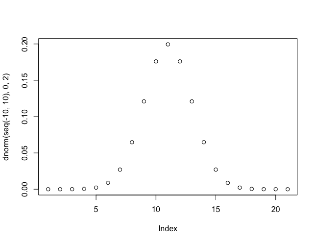
rnorm() 可以生成符合某个分布的随机数,pnorm() 计算出正态分布的累积概率函数:
> rnorm(10, 3, 2)
[1]  2.9455919  5.6487038  0.9341445  2.7948578 -1.5562341  1.6078429
[7]  0.4516596  3.3077327  5.6856195  3.8256133
> pnorm(10, 3, 2)
[1] 0.9997674
其他分布也同理,只需要加上d,p,r即可。
作图
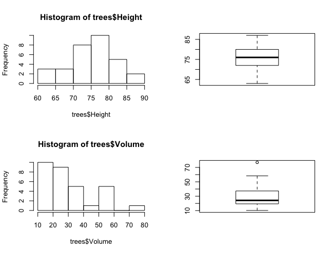
使用 par() 完成 subplot:
> par(mfrow=c(2,2))
> hist(trees$Height)
> boxplot(trees$Height)
> hist(trees$Volume)
> boxplot(trees$Volume)
 使用
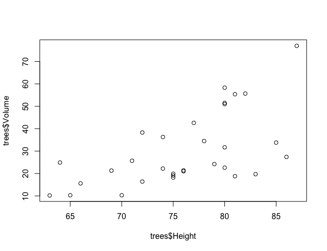
使用 plot() 飞速做出一个最简陋的散点图:
> plot(trees$Height, trees$Volume)
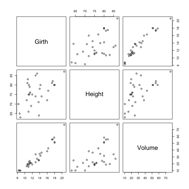
 使用
使用 pairs() 飞速做出 trees 数据集中两两变量之间的关系:
> pairs(trees)
编写函数
如下方法编写自己的函数:
> sd <- function(x) sqrt(var(x))
> x <- c(9, 5, 2, 3, 7)
> sd(x)
[1] 2.863564
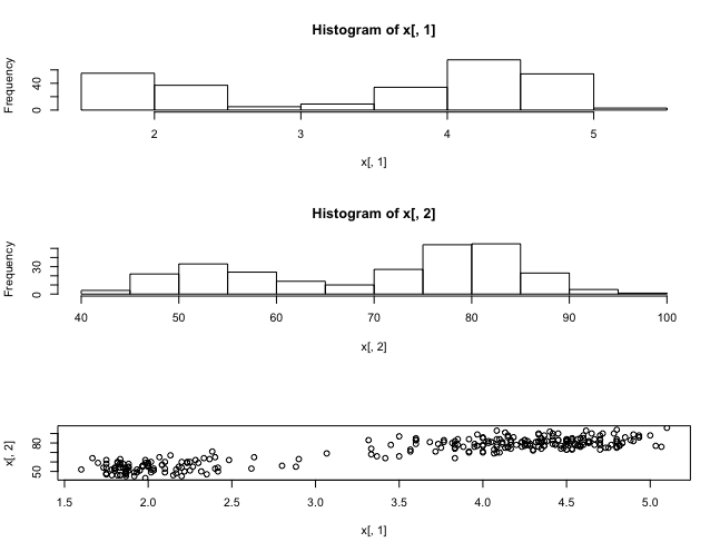
> several.plots <- function (x)
{
par(mfrow=c(3, 1))
hist(x[ ,1])
hist(x[, 2])
plot(x[, 1], x[, 2])
par(mfrow=c(1, 1))
apply(x, 2, summary)
}
> several.plots(faithful)
eruptions waiting
Min. 1.600000 43.00000
1st Qu. 2.162750 58.00000
Median 4.000000 76.00000
Mean 3.487783 70.89706
3rd Qu. 4.454250 82.00000
Max. 5.100000 96.00000
其他
- 如果想退出 R 语言,可以使用
q(); - 如果不明白某个函数的功能,使用
help(func)即可; - 使用
library(libraryname)来载入别的包。