dplyr 包里面必会的处理数据方法
最近沉迷于手游,导致博客久久没有更新。其实博客就是个自己阶段学习的总结,把自己学会的东西写成博客,算是自己复习了一遍,将来忘了的时候也有的看。最近学习的很简单,就是 dplyr 包里面最基础的 5 种数据处理方法。
所用的数据集
这次我们所有数据处理的用法范例都是建立在 flights 数据集上的,先来看看这个数据集:
library(nycflights13)
library(tidyverse)

head(flights)
可以看到,每一条数据代表的是一次航班飞行记录的相关信息:
# A tibble: 6 x 19
   year month   day dep_time sched_dep_time dep_delay arr_time sched_arr_time
  <int> <int> <int>    <int>          <int>     <dbl>    <int>          <int>
1  2013     1     1      517            515         2      830            819
2  2013     1     1      533            529         4      850            830
3  2013     1     1      542            540         2      923            850
4  2013     1     1      544            545        -1     1004           1022
5  2013     1     1      554            600        -6      812            837
6  2013     1     1      554            558        -4      740            728
# ... with 11 more variables: arr_delay <dbl>, carrier <chr>, flight <int>,
#   tailnum <chr>, origin <chr>, dest <chr>, air_time <dbl>, distance <dbl>,
#   hour <dbl>, minute <dbl>, time_hour <dttm>
看看这个数据集中都包含了哪些项目(其中一些项目的含义可以通过名字猜出一二):
> names(flights)
 [1] "year"           "month"          "day"            "dep_time"
 [5] "sched_dep_time" "dep_delay"      "arr_time"       "sched_arr_time"
 [9] "arr_delay"      "carrier"        "flight"         "tailnum"
[13] "origin"         "dest"           "air_time"       "distance"
[17] "hour"           "minute"         "time_hour"
当然在 Rstudio 中,可以更加方便地通过 View(flights) 来查看数据集。
接下来就来说一说 dplyr 最基础的 5 个处理数据的方法:
-
使用
filter()来过滤筛选 -
使用
arrange()来重新排列 -
使用
select()来选择数据集里面的变量 -
使用
mutate(),基于已有的变量,创建需要的新变量 -
使用
summarize()打碎重组多个变量,来完成一些概括
每个函数我都想拿例子来介绍。
观测的「过滤器」:filter()
filter() 筛选的目标是观测(也就是数据中横向的行)。
如果想看看我生日那天的航班数据:
> filter(flights, month == 7, day == 31)
# A tibble: 1,001 x 19
    year month   day dep_time sched_dep_time dep_delay arr_time sched_arr_time
   <int> <int> <int>    <int>          <int>     <dbl>    <int>          <int>
 1  2013     7    31       10           2359        11      344            340
 2  2013     7    31       19           2359        20      355            344
 3  2013     7    31      132           2359        93      510            350
 4  2013     7    31      459            500        -1      633            640
 5  2013     7    31      529            536        -7      755            806
 6  2013     7    31      534            515        19      739            725
 7  2013     7    31      540            540         0      829            840
 8  2013     7    31      541            545        -4      912            921
 9  2013     7    31      542            545        -3      803            813
10  2013     7    31      551            600        -9      640            700
# ... with 991 more rows, and 11 more variables: arr_delay <dbl>, carrier <chr>,
#   flight <int>, tailnum <chr>, origin <chr>, dest <chr>, air_time <dbl>,
#   distance <dbl>, hour <dbl>, minute <dbl>, time_hour <dttm>
看看整个夏天的航班数据(使用逻辑运算符):
> filter(flights, month == 6 | month == 7 | month == 8)
# A tibble: 86,995 x 19
    year month   day dep_time sched_dep_time dep_delay arr_time sched_arr_time
   <int> <int> <int>    <int>          <int>     <dbl>    <int>          <int>
 1  2013     6     1        2           2359         3      341            350
 2  2013     6     1      451            500        -9      624            640
 3  2013     6     1      506            515        -9      715            800
 4  2013     6     1      534            545       -11      800            829
 5  2013     6     1      538            545        -7      925            922
 6  2013     6     1      539            540        -1      832            840
 7  2013     6     1      546            600       -14      850            910
 8  2013     6     1      551            600        -9      828            850
 9  2013     6     1      552            600        -8      647            655
10  2013     6     1      553            600        -7      700            711
# ... with 86,985 more rows, and 11 more variables: arr_delay <dbl>,
#   carrier <chr>, flight <int>, tailnum <chr>, origin <chr>, dest <chr>,
#   air_time <dbl>, distance <dbl>, hour <dbl>, minute <dbl>, time_hour <dttm>
当然更好的方法可能是:
filter(flights, month %in% c(6, 7, 8))
对观测进行重排:arrange()
arrange()的目标也是观测(横向的行),只不过是对观测进行重排。比如我想要以起飞时的延迟时间 dep_delay 的倒序排列:
> arrange(flights, desc(dep_delay))
# A tibble: 336,776 x 19
    year month   day dep_time sched_dep_time dep_delay arr_time sched_arr_time
   <int> <int> <int>    <int>          <int>     <dbl>    <int>          <int>
 1  2013     1     9      641            900      1301     1242           1530
 2  2013     6    15     1432           1935      1137     1607           2120
 3  2013     1    10     1121           1635      1126     1239           1810
 4  2013     9    20     1139           1845      1014     1457           2210
 5  2013     7    22      845           1600      1005     1044           1815
 6  2013     4    10     1100           1900       960     1342           2211
 7  2013     3    17     2321            810       911      135           1020
 8  2013     6    27      959           1900       899     1236           2226
 9  2013     7    22     2257            759       898      121           1026
10  2013    12     5      756           1700       896     1058           2020
# ... with 336,766 more rows, and 11 more variables: arr_delay <dbl>,
#   carrier <chr>, flight <int>, tailnum <chr>, origin <chr>, dest <chr>,
#   air_time <dbl>, distance <dbl>, hour <dbl>, minute <dbl>, time_hour <dttm>
变量的选择器:select()
select() 可以灵活选择数据集中的变量,或者叫特征(纵向的列)。
比如我们只想看日期和起飞时间这几个变量,可以用 year: dep_time 来进行选择:
> select(flights, year:dep_time)
# A tibble: 336,776 x 4
    year month   day dep_time
   <int> <int> <int>    <int>
 1  2013     1     1      517
 2  2013     1     1      533
 3  2013     1     1      542
 4  2013     1     1      544
 5  2013     1     1      554
 6  2013     1     1      554
 7  2013     1     1      555
 8  2013     1     1      557
 9  2013     1     1      557
10  2013     1     1      558
# ... with 336,766 more rows
可以在参数中使用 everything() 来代表所有变量。
如何添加新变量:mutate()
如果基于原有的数据集,想要添加新的变量(纵向的列),mutate() 正是你所需要的的。
比如我们已知航班的飞行时间和飞行距离,就可以计算出航班的平均速度,并添加这个变量:
> mutate(select(flights, year: day, distance, air_time),
+        speed = distance / air_time * 60)
# A tibble: 336,776 x 6
    year month   day distance air_time    speed
   <int> <int> <int>    <dbl>    <dbl>    <dbl>
 1  2013     1     1     1400      227 370.0441
 2  2013     1     1     1416      227 374.2731
 3  2013     1     1     1089      160 408.3750
 4  2013     1     1     1576      183 516.7213
 5  2013     1     1      762      116 394.1379
 6  2013     1     1      719      150 287.6000
 7  2013     1     1     1065      158 404.4304
 8  2013     1     1      229       53 259.2453
 9  2013     1     1      944      140 404.5714
10  2013     1     1      733      138 318.6957
# ... with 336,766 more rows
使用 transmute() 可以只保留新变量。
概括一个数据集:summarize()
说「概括数据集」可能不太合适,summarize() 可以求得某个变量的平均值,总和等统计量。
比如我们求起飞延迟时间的平均值:
> summarize(flights, delay = mean(dep_delay, na.rm = TRUE))
# A tibble: 1 x 1
     delay
     <dbl>
1 12.63907
summarize() 经常和 group_by() 一起用,这样能对原数据集分组并求出想要的统计量:
> flights %>%
+     group_by(year, month, day) %>%
+     summarize(delay = mean(dep_delay, na.rm = TRUE))
# A tibble: 365 x 4
# Groups:   year, month [?]
    year month   day     delay
   <int> <int> <int>     <dbl>
 1  2013     1     1 11.548926
 2  2013     1     2 13.858824
 3  2013     1     3 10.987832
 4  2013     1     4  8.951595
 5  2013     1     5  5.732218
 6  2013     1     6  7.148014
 7  2013     1     7  5.417204
 8  2013     1     8  2.553073
 9  2013     1     9  2.276477
10  2013     1    10  2.844995
# ... with 355 more rows
可以看到,所有观测都被按日期分组了,而 delay 表示的是每组的平均值。这里 na.rm 意思是 remove na,即移除缺失值。
%>% 代表的是一种操作流程(pipeline),这个符号之前的数据集作为符号之后函数的第一个参数。
综合使用
直接拍上下面一段代码,这里用到了 filter(),summarize(),并使用 ggplot 画图。
> library(ggplot)
> flights %>%
+   filter(!is.na(dep_delay), !is.na(arr_delay)) %>%
+   group_by(tailnum) %>%
+   summarize(
+     delay = mean(arr_delay),
+     n = n()
+   ) %>%
+   filter(n > 25) %>%
+   ggplot(mapping = aes(x = n, y = delay)) +
+   geom_point(alpha = 1/10)
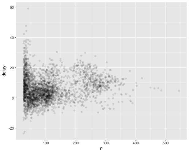
我们先把 dep_delay 和 arr_delay 这两列里面包含 na 值的观测移除掉,以航班尾号分组,查看每组的数量和到达延迟时间,并作图。
这篇虽然只是相当基本地介绍了 5 种函数,但是博客也够长了,就先到这里打住吧。


